이 강좌에 대하여

최근 조회 22,867회

Interested in learning how to solve partial differential equations with numerical methods and how to turn them into python codes? This course provides you with a basic introduction how to apply methods like the finite-difference method, the pseudospectral method, the linear and spectral element method to the 1D (or 2D) scalar wave equation. The mathematical derivation of the computational algorithm is accompanied by python codes embedded in Jupyter notebooks. In a unique setup you can see how the mathematical equations are transformed to a computer code and the results visualized. The emphasis is on illustrating the fundamental mathematical ingredients of the various numerical methods (e.g., Taylor series, Fourier series, differentiation, function interpolation, numerical integration) and how they compare. You will be provided with strategies how to ensure your solutions are correct, for example benchmarking with analytical solutions or convergence tests. The mathematical aspects are complemented by a basic introduction to wave physics, discretization, meshes, parallel programming, computing models. 
The course targets anyone who aims at developing or using numerical methods applied to partial differential equations and is seeking a practical introduction at a basic level. The methodologies discussed are widely used in natural sciences,  engineering, as well as economics and other fields.

유연한 마감일

일정에 따라 마감일을 재설정합니다.

공유 가능한 수료증

완료 시 수료증 획득

100% 온라인

지금 바로 시작해 나만의 일정에 따라 학습을 진행하세요.

중급 단계

Basic knowledge of calculus and analysis, series, partial differential equations, and linear algebra.

완료하는 데 약 35시간 필요

영어

자막: 프랑스어, 포르투갈어 (유럽), 러시아어, 영어, 스페인어

배울 내용

How to solve a partial differential equation using the finite-difference, the pseudospectral, or the linear (spectral) finite-element method.
Understanding the limits of explicit space-time simulations due to the stability criterion and spatial and temporal sampling requirements.
Strategies how to plan and setup sophisticated simulation tasks.
Strategies how to avoid errors in simulation results.

유연한 마감일

일정에 따라 마감일을 재설정합니다.

공유 가능한 수료증

완료 시 수료증 획득

100% 온라인

지금 바로 시작해 나만의 일정에 따라 학습을 진행하세요.

중급 단계

Basic knowledge of calculus and analysis, series, partial differential equations, and linear algebra.

완료하는 데 약 35시간 필요

영어

자막: 프랑스어, 포르투갈어 (유럽), 러시아어, 영어, 스페인어

강사

강사 평가

4.86/5 (106개의 평가)

Heiner Igel

Prof. Dr.

Earth and Environmental Sciences

17,506명의 학습자

1개의 강좌

강의 계획표 - 이 강좌에서 배울 내용

콘텐츠 평가97%(1,522개의 평가)

주

1

주 1

완료하는 데 3시간 필요

Week 01 - Discrete World, Wave Physics, Computers

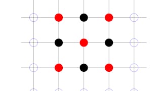
The use of numerical methods to solve partial differential equations is motivated giving examples form Earth sciences. Concepts of discretization in space and time are introduced and the necessity to sample fields with sufficient accuracy is motivated (i.e. number of grid points per wavelength). Computational meshes are discussed and their power and restrictions to model complex geometries illustrated. The basics of parallel computers and parallel programming are discussed and their impact on realistic simulations. The specific partial differential equation used in this course to illustrate various numerical methods is presented: the acoustic wave equation. Some physical aspects of this equation are illustrated that are relevant to understand its solutions. Finally Jupyter notebooks are introduced that are used with Python programs to illustrate the implementation of the numerical methods.

완료하는 데 3시간 필요

6개 동영상 (총 63분), 1 개의 읽기 자료, 1 개의 테스트

주

2

주 2

완료하는 데 4시간 필요

Week 02 The Finite-Difference Method - Taylor Operators

In Week 2 we introduce the basic definitions of the finite-difference method. We learn how to use Taylor series to estimate the error of the finite-difference approximations to derivatives and how to increase the accuracy of the approximations using longer operators. We also learn how to implement numerical derivatives using Python.

완료하는 데 4시간 필요

8개 동영상 (총 41분)

주

3

주 3

완료하는 데 3시간 필요

Week 03 The Finite-Difference Method - 1D Wave Equation - von Neumann Analysis

We develop the finite-difference algorithm to the acoustic wave equation in 1D, discuss boundary conditions and how to initialize a simulation example. We look at solutions using the Python implementation and observe numerical artifacts. We analytically derive one of the most important results of numerical analysis – the CFL criterion which leads to a conditionally stable algorithm for explicit finite-difference schemes.

완료하는 데 3시간 필요

9개 동영상 (총 50분)

주

4

주 4

완료하는 데 7시간 필요

Week 04 The Finite-Difference Method in 2D - Numerical Anisotropy, Heterogeneous Media

We develop the solution to the 2D acoustic wave equation, compare with analytical solutions and demonstrate the phenomenon of numerical (non-physical) anisotropy. We extend the von Neumann Analysis to 2D and derive numerical anisotropy analytically. We learn how to initialize a realistic physical problem and illustrate that 2D solution are already quite powerful to understand complex wave phenomena. We introduced the 1D elastic wave equation and show the concept of staggered-grid schemes with the coupled first-order velocity-stress formulation.

완료하는 데 7시간 필요

10개 동영상 (총 83분)

10개의 동영상

W4V1 Acoustic Waves 2D – Analytical Solutions8m

W4V2 Acoustic Waves 2D – Finite-Difference Algorithm6m

W4V3 Python: Acoustic Waves 2D8m

W4V4 Acoustic Waves 2D – von Neumann Analysis5m

W4V5 Acoustic Waves 2D – Waves in a Fault Zone8m

W4V6 Python: Waves in a Fault Zone9m

W4V7 Elastic Wave Equation – Staggered Grids16m

W4V8 Python: Staggered Grids5m

W4V9 Improving numerical accuracy11m

W4V10 Wrap up3m

1개 연습문제

Acoustic Wave Equation in 2D - Numerical Anisotropy - Staggered Grids45m

주

5

주 5

완료하는 데 6시간 필요

Week 05 The Pseudospectral Method, Function Interpolation

We start with the problem of function interpolation leading to the concept of Fourier series. We move to the discrete Fourier series and highlight their exact interpolation properties on regular spatial grids. We introduce the derivative of functions using discrete Fourier transforms and use it to solve the 1D and 2D acoustic wave equation. The necessity to simulate waves in limited areas leads us to the definition of Chebyshev polynomials and their uses as basis functions for function interpolation. We develop the concept of differentiation matrices and discuss a solution scheme for the elastic wave equation using Chebyshev polynomials.

완료하는 데 6시간 필요

9개 동영상 (총 62분)

9개의 동영상

W5V1 Function Interpolation – Trigonometric basis functions5m

W5V2 Fourier Series - Examples5m

W5V3 Discrete Fourier Series5m

W5V4 The Fourier Transform - Derivative6m

W5V5 Solving the 1D/2D Wave Equation with Python11m

W5V6 Convolutional Operators6m

W5V7 Chebyshev Polynomials - Derivatives8m

W5V8 Chebyshev Method – 1D Elastic Wave Equation7m

W5V9 Summary3m

1개 연습문제

Pseudospectral method45m

주

6

주 6

완료하는 데 2시간 필요

Week 06 The Linear Finite-Element Method - Static Elasticity

We introduce the concept of finite elements and develop the weak form of the wave equation. We discuss the Galerkin principle and derive a finite-element algorithm for the static elasticity problem based upon linear basis functions. We also discuss how to implement boundary conditions. The finite-difference based relaxation method is derived for the same equation and the solution compared to the finite-element algorithm.

완료하는 데 2시간 필요

5개 동영상 (총 42분)

주

7

주 7

완료하는 데 3시간 필요

Week 07 The Linear Finite-Element Method - Dynamic Elasticity

We extend the finite-element solution to the elastic wave equation and compare the solution scheme to the finite-difference method. To allow direct comparison we formulate the finite-difference solution in matrix-vector form and demonstrate the similarity of the linear finite-element method and the finite-difference approach. We introduce the concept of h-adaptivity, the space-dependence of the element size for heterogeneous media.

완료하는 데 3시간 필요

7개 동영상 (총 56분)

주

8

주 8

완료하는 데 4시간 필요

Week 08 The Spectral-Element Method - Lagrange Interpolation, Numerical Integration

We introduce the fundamentals of the spectral-element method developing a solution scheme for the 1D elastic wave equation. Lagrange polynomials are discussed as the basis functions of choice. The concept of Gauss-Lobatto-Legendre numerical integration is introduced and shown that it leads to a diagonal mass matrix making its inversion trivial.

완료하는 데 4시간 필요

7개 동영상 (총 51분)

주

9

주 9

완료하는 데 4시간 필요

Week 09 The Spectral Element Method - 1D Elastic Wave Equation, Convergence Test

We finalize the derivation of the spectral-element solution to the elastic wave equation. We show how to calculate the required derivatives of the Lagrange polynomials making use of Legendre polynomials. We show how to perform the assembly step leading to the final solution system for the elastic wave equation. We demonstrate the numerical solution for homogenous and heterogeneous media.

완료하는 데 4시간 필요

7개 동영상 (총 50분)

검토

4.7

110개의 리뷰

5 stars
80.20%
4 stars
15.77%
3 stars
2.01%
2 stars
1.67%
1 star
0.33%